Inside the Wan2.2 VAE Decoder
A detailed explanation of the decoder’s architecture and operations.
October 23, 2026
Introduction
A variational autoencoder (VAE) consists of an encoder and a decoder. The encoder compresses images or videos into latents, while the decoder reconstructs the original input from these latents. Because this compression is lossy, the reconstructed pixels approximate the original input, as illustrated in Figure 1.

Scroll figures sideways to see the full diagram.
VAEs in Video Generation
In text-to-video generation, the diffusion model operates in latent space, reducing the computation required compared to generating pixels directly. Starting from noise, it repeatedly denoises the latents conditioned on the text prompt. The VAE decoder then converts the resulting latents into RGB frames. As shown in Figure 2, the decoder receives its input from the diffusion model rather than the VAE encoder.
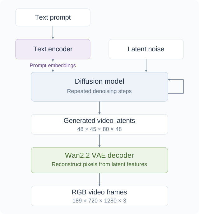
Cosmos3-Nano uses the Wan2.2 VAE from Wan2.2-TI2V-5B.
Decoder Architecture
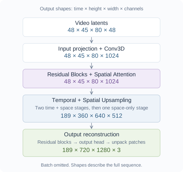
Figure 3 shows the decoder stages for a 720p video with 189 frames.
Input Projection
The decoder first reverses the latent normalization and applies a 1 × 1 × 1 Conv3D projection. At each position, this projection computes a learned linear combination of the 48 input channels to produce 48 output channels. Because the kernel spans only one position, it mixes channels without reading neighboring positions or changing the tensor shape.
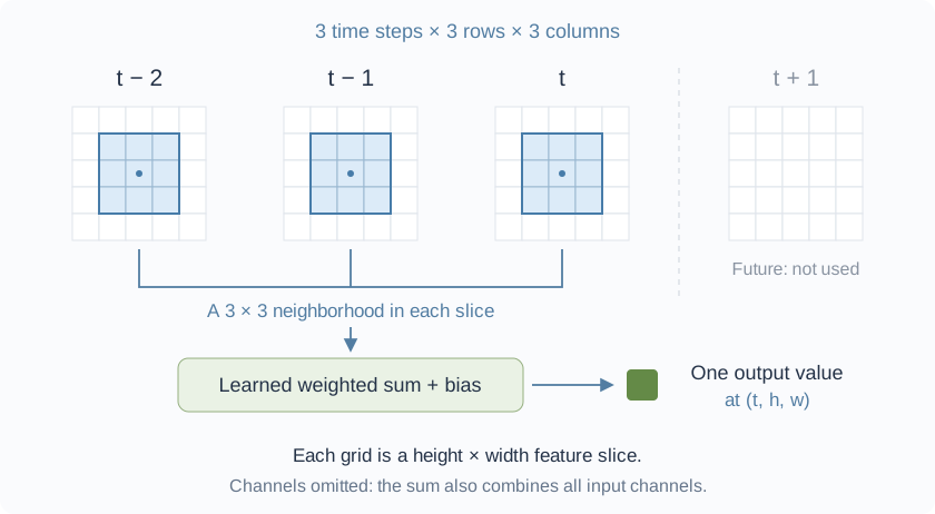
A 3 × 3 × 3 causal Conv3D then expands the channel dimension from 48 to 1,024, preserving the 48 × 45 × 80 grid. With kernel dimensions ordered as time × height × width, each output combines a 3 × 3 spatial neighborhood from the current and two preceding time steps. Restricting the temporal window to current and past inputs makes the convolution causal. Missing earlier inputs are padded with zeros. Figure 4 illustrates these dependencies.
Residual Blocks and Spatial Attention
Before upsampling, the decoder applies two residual blocks with spatial attention between them, as shown in Figure 5. These operations preserve the 48 × 45 × 80 × 1024 shape while combining information from neighboring positions through convolutions and across the spatial grid through attention.
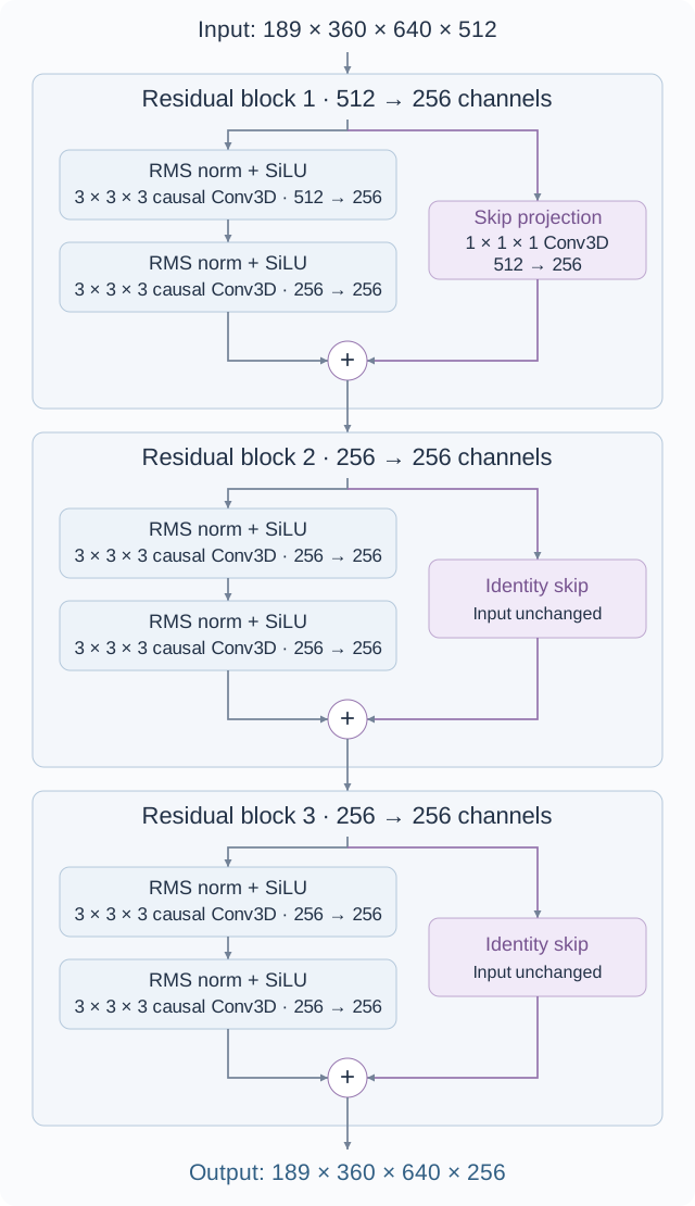
Each residual block applies two sequences of RMS normalization, SiLU, and causal Conv3D, then adds the skip connection.
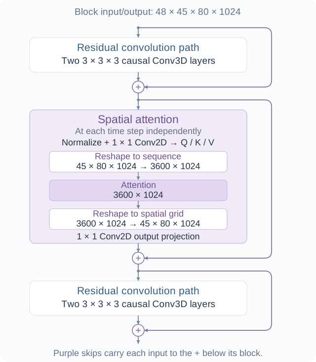
Spatial attention operates independently at each time step. After normalization, a 1 × 1 Conv2D projects the 1,024 input channels into queries, keys, and values, each with 1,024 channels. The 45 × 80 spatial grid is then flattened into 3,600 positions for attention. The attention output is reshaped back to the grid and projected through a final 1 × 1 Conv2D, before adding the block’s input through the skip connection.
Temporal and Spatial Upsampling
Temporal upsampling increases the number of time steps, while spatial upsampling increases height and width at each time step. Both operate on intermediate features, which are not yet RGB frames.
Three stages expand the feature grid from 48 × 45 × 80 × 1024 to 189 × 360 × 640 × 512. The first two expand time and space, while the third expands only space. Each stage contains residual blocks, upsampling, and a skip connection, as shown in Figure 6.
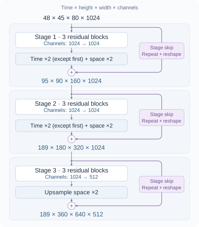
Each stage begins with three residual blocks that preserve the temporal and spatial dimensions. In the third stage, the first block also reduces the channel dimension from 1,024 to 512, requiring a learned projection on its skip connection. The remaining blocks preserve the channel dimension and therefore use identity skip connections.
Temporal upsampling uses a 3 × 1 × 1 causal Conv3D to predict twice as many channels at each spatial position, providing the values for both output steps. Reshaping separates these values into two time steps, each with the original channel count. For example, with two channels per step:
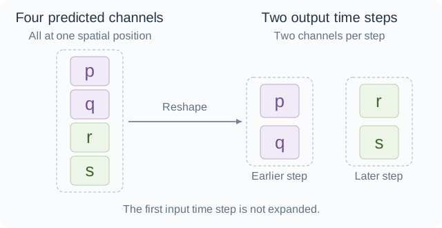
The two output steps can have different values because the convolution predicts them separately. Since the first input step is not expanded, a stage with T input steps produces 1 + 2(T − 1) output steps. The two temporal upsampling stages therefore increase the sequence length from 48 → 95 → 189 steps.
Spatial upsampling enlarges the feature grid at each time step without changing the number of time steps. Nearest-neighbor resizing copies each feature vector into a 2 × 2 area, doubling height and width—for example, from 45 × 80 → 90 × 160. A 3 × 3 Conv2D then mixes neighboring features within each time step. All three stages perform spatial upsampling, increasing the grid from 45 × 80 → 90 × 160 → 180 × 320 → 360 × 640. In the first two stages, this follows temporal upsampling.
The Repeat-and-Reshape Skip Connection
In addition to the skip connections within individual residual blocks, each stage has a stage skip connection, shown in purple in Figure 6. This branch bypasses both the residual blocks and the upsampling operations. To make its output compatible with the main branch, it repeats and rearranges channel values without learned weights. The two branches are then added elementwise.
Stages 1 and 2: expand time and space.
At one input position, each channel value a is repeated across four spatial positions at each of two consecutive output time steps. This produces two 2 × 2 patches with the same channel count:
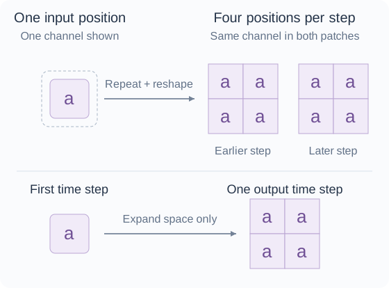
This operation is applied independently to each of the 1,024 channels, matching the spatial and temporal expansion of the main branch.
Stage 3: expand space and halve the channels.
At each spatial position, the skip connection takes a pair of input channels and maps their values into one output channel’s 2 × 2 patch. If the two values are a and b, repeating each value twice fills the patch as follows:
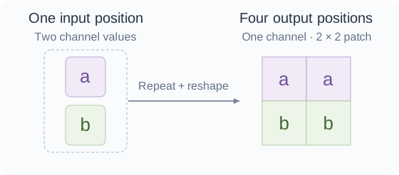
Each pair of input channels therefore becomes one output channel spread across four spatial positions. This halves the channel count from 1,024 to 512 while doubling height and width. The number of time steps stays unchanged.
Both input values are preserved in the patch, with no averaging or learned weights. The main branch reaches the same output shape through its convolutions and spatial upsampling, allowing the two branches to be added.
Output Reconstruction
At this point, each position in the 189 × 360 × 640 grid contains 512 feature values. Output reconstruction converts these features into RGB pixels. It first reduces the channel count, then predicts the values for four pixels at each position, and finally arranges those pixels into the full-resolution frames.
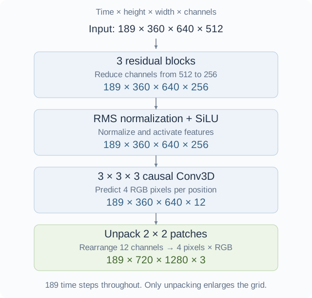
The output head applies RMS normalization, SiLU, and a 3 × 3 × 3 causal Conv3D to predict 12 values at each grid position: the RGB values for four pixels. Unpacking then rearranges the 12 predicted values at each position into a 2 × 2 patch of RGB pixels, doubling height and width without changing the number of frames.
Final Residual Blocks
The final three residual blocks reduce the channel count from 512 to 256, keeping the number of time steps, height, and width unchanged. The first block performs this reduction in its first convolution and uses a 1 × 1 × 1 Conv3D on the skip connection to match. The remaining convolutions preserve 256 channels, and the next two blocks use identity skip connections.
References
- Wan2.2 VAE implementation: decoder architecture, convolutions, attention, upsampling, and repeat-and-reshape skip connections.
- Cosmos3-Nano VAE configuration: the Wan2.2 model configuration used for this article.